Bringing risk-awareness to general-utility MDPs

Abstract

The framework of general-utility MDPs generalizes objective-specification beyond standard MDPs by considering an objective function that depends non-linearly on the frequency of visitation of states induced by a given policy. For example, general-utility MDPs can be used to encode imitation or exploration tasks, which cannot be easily encoded by specifying a reward/cost signal. In this blog post, we motivate risk-aware general-utility MDPs, where we aim to find an optimal policy with respect to a risk measure of the distribution of objective values induced by its interaction with the MDP. We also show how we can find such an optimal policy by resorting to online planning techniques.

The contents of this blog post are based on the following article

@article{santos2026riskaware,
    title={Risk-Aware General-Utility Markov Decision Processes},
    author={Pedro Pinto Santos and Fábio Vital and Alberto Sardinha and Francisco S. Melo},
    journal={Reinforcement Learning Journal},
    volume={7},
    pages={},
    year={2026}
}

Disclaimer

No LLMs were involved in the creation of this blog post.

1) Motivating example: Exploring three rooms

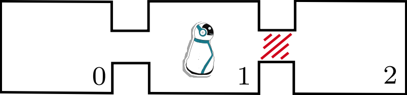
Assume an agent (robot) in an environment comprising three rooms as illustrated below. The agent can move between adjacent rooms by traversing two corridors. The agent aims to visit all rooms as uniformly as possible. This kind of objective is relevant in the context of exploration tasks, where an agent may want to explore the environment without being focused on optimizing any particular cost function.

We can easily resort to the framework of general-utility MDPs (GUMDPs) to encode the exploration task of visiting all rooms as uniformly as possible. This is because in GUMDPs the performance of a given policy depends on its induced frequency of visitation of states.

In particular, a GUMDP is defined by the tuple

$$(\mathcal{S}, \mathcal{A}, (P^a : \forall a \in \mathcal{A}) , p_0, f, \gamma),$$

such that we can let the set of states $\mathcal{S}$ to be the different rooms, the set of actions $\mathcal{A}$ corresponds to the transitions between the rooms, and we can also specificy a distribution of initial states $p_0$ as well as a set of transition probability matrices $P^a$ to encode the dynamics of the environment. Finally, as in GUMDPs, we aim to find

$$\pi^* \in \text{argmin}_\pi f(d_\pi),$$

where $d_\pi \in \mathbb{R}^{|\mathcal{S}||\mathcal{A}|}$ is the discounted state-action frequency visitation (also known as occupancy), entry-wise defined as

and $\gamma \in [0,1)$ is a discount factor.

Then, letting $f(d) = d^\top \log(d)$, i.e., (minus) the entropy function, encodes our objective of visiting the rooms of the environment as uniformly as possible.

We refer to From MDPs to general-utility MDPs for more details regarding the GUMDPs framework.

2) Why risk-awareness matters in GUMDPs

Consider again the same environment above described, where an agent (robot) aims to explore three rooms as uniformly as possible, reproduced below for improved readability.

We now add an important detail about the environment. Transitioning from room 0 to room 1 incurs no danger to the robot. However, attempting to transition from room 1 to room 2 may cause irreparable damage to the robot, rendering it unable to explore the environment further (illustrated by the red stripes in the figure above).

The dynamics of this environment are abstracted below, where each state corresponds to one of the rooms, the actions encode the transitions between rooms, and $\epsilon \in (0,1)$ is the probability of irreparable damage to the robot when attempting to transition from room 1 to room 2. Similar to the previous section, our objective function $f$ corresponds to (minus) the entropy of the discounted frequency of visitation of states induced by any policy.

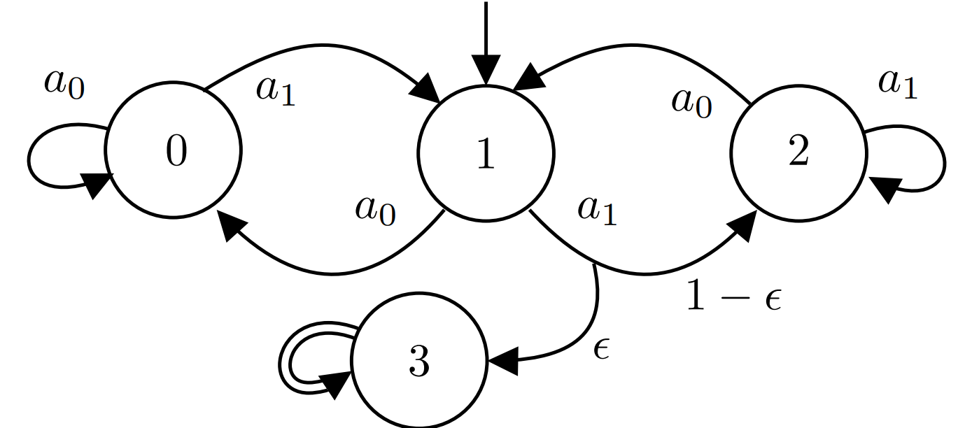
Now, from perspective of the agent, it is not totally clear whether the agent should attempt to visit room 2 since there is a chance it may suffer irreparable damage, not being able to further explore the environment. On the one hand, if the agent is optimistic, then it should try to transition between room 1 and 2 because there is a chance it succeeds (with probability $1-\epsilon$), yielding the best possible outcome - being able to explore all three rooms. On the other hand, if the agent is pessimistic, it should not attempt to transition between room 1 and 2 because there is a chance it fails (with probability $\epsilon$), hence getting stuck and not able to further explore the environment. Therefore, depending on the risk-level the agent is willing to accept, the optimal policy may be different.

To further illustrate why different policies may lead to very different outcomes in context of the environment above, consider two policies:

• Policy 1 ($\pi_1$), a risk-seeking policy that attempts to visit all rooms, including room 2; and
• Policy 2 ($\pi_2$), a risk-averse policy that does not attempt to visit room 2 and, instead, keeps alternating between rooms 0 and 1.

The plot below shows the density¹ of the objective values, in this case the entropy of the discounted occupancy induced by each of the policies. Both policies yield very different distributions, with the risk-seeking policy $\pi_1$ attaining lower (better) objective values at the cost of sometimes obtaining higher (worse) objective values. On the other hand, the risk-averse policy $\pi_2$ always attains the same intermediate objective value due to its deterministic behavior.

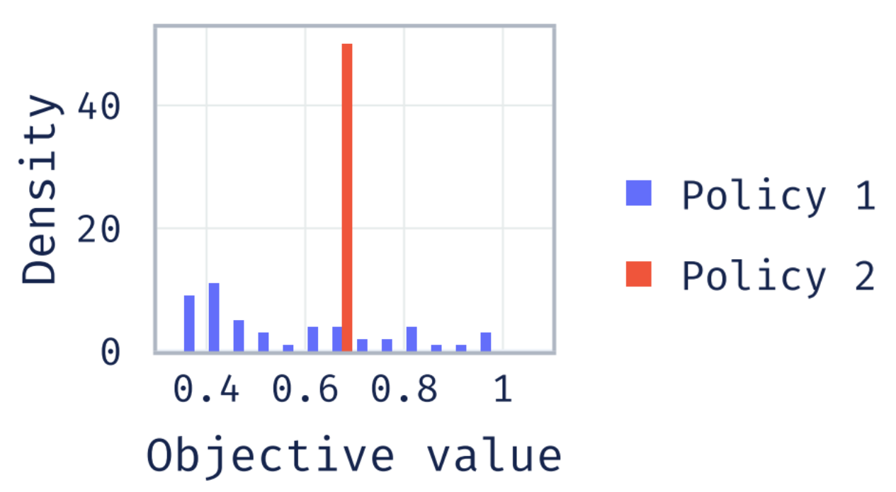
Thus, depending on the risk-level the agent is willing to accept, the preferred policy may differ.

In the next section, we introduce and formalize risk-aware GUMDPs, where we aim to find the optimal policy with respect to a risk measure of the distribution of objective values induced by any policy.

3) Towards risk-aware GUMDPs

For a given random trajectory $\omega = (\mathrm{s}_0, \mathrm{a}_0, \mathrm{s}_1, \mathrm{a}_1, \ldots )$, we let its associated random occupancy vector $\mathbf{\mathrm{d}}^\pi \in \mathbb{R}^{|\mathcal{S}||\mathcal{A}|}$ be defined, for each $(s,a)$ entry, as

We then aim to find the optimal policy

$$\pi^* \in \text{argmin}_\pi \rho(f(\mathrm{d}^\pi)),$$

where $\rho$ is a risk measure computed over the random objective. Risk measures quantify an agent’s attitude toward uncertainty and variability in outcomes. The risk-aware objective allows the agent to reason over the entire distribution instead of just its expectation (particular case where $\rho(\cdot) = \mathbb{E}[\cdot]$).

In the context of our work, we focus our attention to the entropic risk measure (ERM). The ERM of a random variable $\mathrm{z}$ is defined as

$$\text{ERM}_\beta(\mathrm{z}) = \frac{1}{\beta} \ln\left( \mathbb{E}\left[\exp(\beta \mathrm{z})\right]\right),$$

where parameter $\beta \in (0, \infty)$ trades off between risk-neutral (expected) performance as $\beta \rightarrow 0$ and risk-aversion as $\beta$ increases.

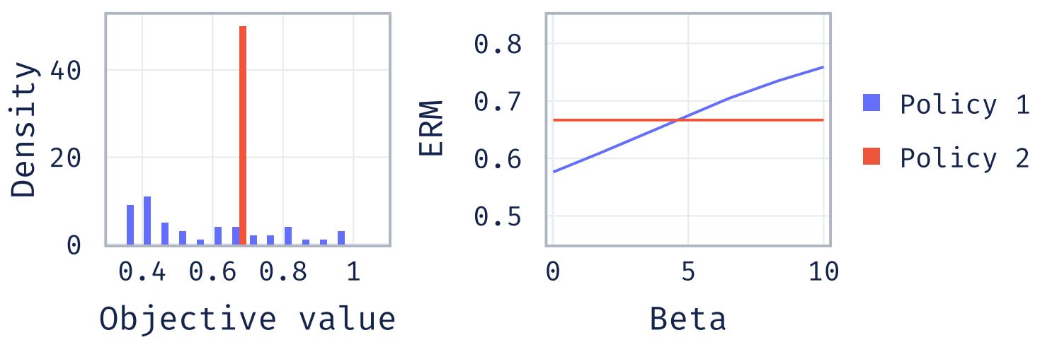
We illustrate below the ERM (right side plot) for the two policies ($\pi_1$ and $\pi_2$) from the exploration motivating example. We recall that $\pi_1$ is risk-seeking as it attempts to visit the three rooms, whereas $\pi_2$ is risk-averse as it does not attempt visiting room 2. As can be seen (lower values are better), for lower $\beta$ (risk-neutral preference) $\pi_1$ is preferred to $\pi_2$. Conversely, for higher $\beta$ (risk-averse preference), $\pi_2$ becomes the preferred policy.

In the next section, we briefly explore how we can solve risk-aware GUMDPs.

4) Solving risk-aware GUMDPs

Solving risk-aware GUMDPs is hard. This is because, even in the case where $\rho(\cdot) = \mathbb{E}[\cdot]$, our problem is already quite hard. Essentially, solving

$$\pi^* \in \text{argmin}_\pi \mathbb{E}[f(\mathrm{d}^\pi)],$$

i.e., the case where $\rho(\cdot) = \mathbb{E}[\cdot]$, is known as the single-trial optimization regime for GUMDPs. We note that this problem is different from solving

$$\pi^* \in \text{argmin}_\pi f(\mathbb{E}[\mathrm{d}^\pi]) \Leftrightarrow \pi^* \in \text{argmin}_\pi f(d_\pi)$$

for which previous works provide different approaches, given that $f$ may be non-linear (hence we cannot swap $f$ with the expectation).

Previous works explored single-trial optimization in the context of GUMDPs (Mutti, 2022) (Santos 1, 2026). In particular, we highlight that we may require non-Markovian (history-dependent) policies for optimality and that the associated decision problem is NP-Hard. Consequently, risk-aware GUMDPs inherit these challenges.

Nevertheless, following similar approaches to previous works (Santos 1, 2026), we show that we can solve any risk-aware GUMDP, up to any accuracy, by:

1. Converting the risk-aware GUMDP into a finite-horizon risk-aware MDP, known as the occupancy MDP, in which the agent keeps track of the accrued occupancy up to any timestep: This MDP has a terminal cost which corresponds to the objective function evaluated at the accrued occupancy, such that optimizing for any risk measure over the distribution of objective values in the original GUMDP is equivalent to optimizing for the same risk measure over the distribution of returns in the occupancy MDP.
2. Applying an online planning approach based on a risk-aware Monte Carlo tree search algorithm to compute approximately optimal policies for the occupancy MDP derived from the original GUMDP: Since the occupancy MDP has an exponential number of states we cannot perform offline planning and, instead, propose an online planning approach where approximately optimal actions are computed for the states encountered in the actual sampled trajectories of interaction with the environment. We consider the entropic risk-aware Monte Carlo tree search algorithm proposed in (Santos 2, 2026) to compute approximately optimal actions at each timestep.

5) Experimental results

We now present some results obtained by our online planning MCTS-based approach to solve risk-aware GUMDPs. We present results for a maximum-state entropy exploration task and a multi-objective task with a non-linear utility function. We refer to our article for additional results under cost minimization, imitation learning, exploration and multi-objective cost minimization tasks.

Exploring a grid-world

Similar to the motivating example, an agent aims to explore the grid-world illustrated below as uniformly as possible. In the environment below, we distinguish between two types of grid cells:

• gray grid cells are standard grid cells posing no danger to the agent.
• at black grid cells, there is a chance the agent gets stuck.

Hence, depeding on the risk-level the agent is willing to accept, the agent should reason whether it is worth to attempt visiting the black cells at the cost of sometimes getting stuck or, instead, explore the environment more conservatively while avoiding such sticky (black) grid cells.

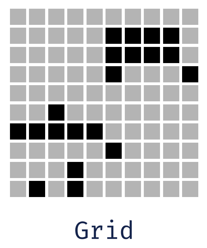
To encode such an objective, we set the objective function, for any occupancy vector $d$, as $f(d) = d^\top \log(d)$, i.e., (minus) the entropy function.

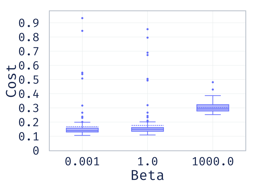
We plot below the distribution of objective values obtained by our risk-aware MCTS-based approach bor different $\beta$ values. As seen:

• for low $\beta$ values, where we are optimizing for risk-neutral behavior, the distribution is more spread apart; but
• as $\beta$ increases and we focus on computing risk-averse behavior, the distribution concentrates around its median, showing that the algorithm is successful in greatly reducing the number of outliers (points with high cost values in the plot).

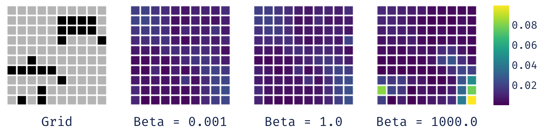
Qualitatively, the plot below displays an heatmap of the cells visited by the agent at execution time for different $\beta$ values. As seen, for low $\beta$ values the agent aims to visit all cells of the environment, whereas for higher $\beta$ values the agent focuses more on cells that are farther away from the sticky (black) grid cells.

Multi-objective resource gathering

An agent in a grid-world aims to retrieve two resources ($R_1$ and $R_2$) back to the agent’s starting position, while avoiding enemies present at specific squares. The environment is slippery in the sense that with a certain probability the agent’s selected action at each timestep fails and, instead, the agent moves perpendicularly to the selected direction.

Each resource is associated with a different cost function:

• the agent receives a cost, given by cost function $c_1$, when failing to deliver $R_1$ to the initial position;
• the agent receives a cost, given by cost function $c_2$, when failing to deliver $R_2$ to the initial position;
• the agent receives a cost, given by cost function $c_3$, when getting defeated by an enemy $(E)$, which happens when visiting a square containing an enemy.

Letting $c_1$, $c_2$, and $c_3$ be the vectorized costs for the different objectives, we set the objective to $f(d) = g(c_1^\top d, c_2^\top d, c_3^\top d)$ such that the non-linear utility function $g$ prioritizes retrieving $R_1$ in comparison to $R_2$. This corresponds to a multi-objective task with a non-linear utility function. We illustrate the environment below.

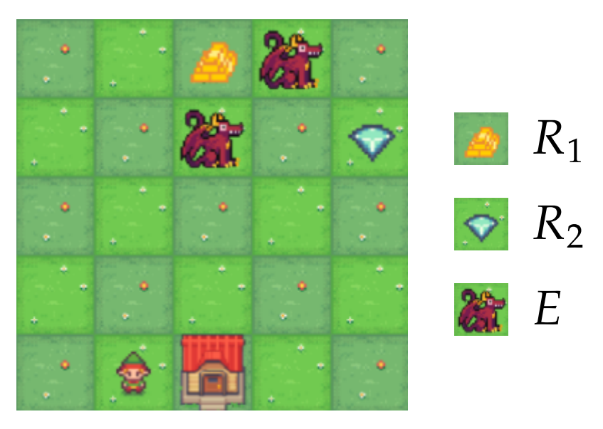
As seen above, retrieving $R_1$ is associated with a higher risk due to its proximity to enemies, whereas $R_2$ is farther away from the enemies and, therefore, a safer choice. Hence, depeding on the risk-level the agent is willing to accept, the agent should reason whether it should aim to retrieve only $R_1$, only $R_2$, or both resources.

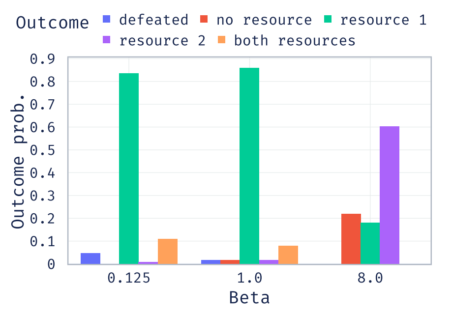
We plot below the outcome probability of different events for different $\beta$ values as obtained by our risk-aware MCTS algorithm. As seen:

• for low $\beta$ values, where we are optimizing for risk-neutral behavior, the agent mostly focuses on the most risky but more valuable resource $R_1$, at the cost of sometimes getting defeated by the enemies; but
• as $\beta$ increases and we focus on computing risk-averse behavior, the agent prefers to retrieve the safer but less valuable resource $R_2$, never getting defeated by the enemies.

Acknowledgments

The authors thank the lab managers at GAIPS for the support provided when running the computational experiments of this work. The authors also thank Jacopo Silvestrin for discussions on earlier versions of this work.

References

(Mutti, 2022) Mutti, M., Santi, R. D., Bartolomeis, P. D., & Restelli, M. (2022). Challenging Common Assumptions in Convex Reinforcement Learning. CoRR, abs/2202.01511.
(Santos 1, 2026) Santos, P. P., Sardinha, A., & Melo, F. S. (2026). Solving General-Utility Markov Decision Processes in the Single-Trial Regime with Online Planning. arXiv [Cs.LG].
(Santos 2, 2026) Santos, P. P., Silvestrin, J., Sardinha, A., & Melo, F. S. (2026). Entropic Risk-Aware Monte Carlo Tree Search. arXiv [Cs.LG].
This distribution plays a similar role to the distribution of discounted returns in the context of distributional RL. In fact, if the objective $f$ is a linear function of the type $f(d_\pi) = d_\pi^\top c$, then the distribution precisely matches the distribution of discounted returns, where $c$ is the vectorized cost function. However, in this work we allow the objective $f$ to depend non-linearly on the occupancy $d_\pi$. ↩︎