From MDPs to general-utility MDPs

Abstract

We explore how general-utility Markov decision processes (GUMDPs) can encode a more rich set of objectives than those considered by the framework of MDPs (with stationary cost functions). We also briefly review connections between GUMDPs and the dual formulation for MDPs, relevant objectives for GUMDPs, and how to solve GUMDPs.

Disclaimer

No LLMs were involved in the creation of this blog post.

1) Why do we need to go beyond MDPs?

The question of whether MDPs suffice to encode all desired objectives is tightly related to the question of whether a cost¹ signal is “enough” for intelligent behavior: Are costs enough? Previous works answered this question in different ways (Silver, 2021) (Vamplew, 2021).

In this work, we do not seek to answer such a question but mostly to understand, from a modeling point-of-view, whether we may want an agent to exhibit certain behavior(s) that cannot be easily encoded via the specification of a cost function. We argue that, yes, there may be interesting and relevant behavior(s) we may want an agent to pursue that cannot be easily specified with a (stationary) cost function.

Motivating example

Assume an agent (robot) in a grid-world environment as illustrated below. The agent can move between adjacent cells depending on the selected actions and, for simplicity, we can assume the environment is deterministic.

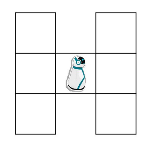
We can model such an environment using the framework of MDPs by letting the set of states $\mathcal{S}$ to be the grid-cell positions, the set of actions $\mathcal{A}$ corresponds to the cardinal directions, and we can also easily specificy a set of transition probability matrices $P^a$, one of each action $a \in \mathcal{A}$, to encode the dynamics of the environment.

A stationary cost function $c$, in its simplest case, maps states to real-valued numbers. For simplicity, we can assume a discount factor $\gamma$ such that the agent aims to minimize the expected sum of discounted costs yielded by the interaction between the agent’s policy $\pi$ and the MDP.

Now, depending on the cost function definition, different optimal behaviors will emerge. We illustrate this below with three possible cost functions, where in each picture the cost funcion is given by the red numbers and the respective induced optimal behavior ($\pi^*$) by the red arrow.

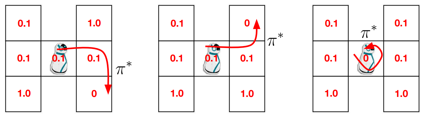
As seen, the optimal behavior induced by any cost function for the MDP above is to move towards the state that has the lowest cost overall and then stay at the state for as long as possible.

However, let’s imagine we want the agent to visit all states as randomly/uniformly as possible. This kind of objective is relevant in the context of exploration tasks, where we may want an agent to explore the environment without being focused on optimizing any particular cost function. Unfortunately, this behavior does not correspond to the optimal behavior induced by any (stationary) cost function². This is because we do not want the agent to move towards any particular state(s) but rather to keep exploring all states as randomly/uniformly as possible.

Let’s think about our problem in a different way. Assume we deploy our agent to the environment with a given policy $\pi$. After a certain number of timesteps, we can calculate the frequency of visition of states induced by the policy, denoted by $d_\pi$. Now, if our objective fuction $f$ depends on this frequency of visitation of states, letting $f$ to be (minus) the entropy function yields precisely our objective of visiting the states of the environment as randomly/uniformly as possible.

This is the key idea behind GUMDPs, i.e., defining objective functions $f$ that depend on the frequency of visitation of states. We will also see that GUMDPs are more general than standard MDPs since we can recover a standard MDP by defining our objective function $f$ in a particular way.

Next, we formally define a GUMDP, starting from the dual formulation for MDPs.

2) From the dual formulation of MDPs to GUMDPs

A Markov decision process is defined by the tuple

$$(\mathcal{S}, \mathcal{A}, (P^a : \forall a \in \mathcal{A}) , p_0, c, \gamma),$$

where $\mathcal{S}$ is the state space, $\mathcal{A}$ the action space, $(P^a : \forall a \in \mathcal{A})$ the tuple of transition matrices, $p_0$ the distribution of initial states, $c : \mathcal{S} \times \mathcal{A} \rightarrow \mathbb{R}$ the cost function, and $\gamma \in [0,1)$ a discount factor. A common objective is to find the optimal policy $\pi^*$ according to the expected sum of discounted costs objective $J(\pi)$, defined as

It holds that

where (a) follows since the sum is convergent, and in (b) we consider vectorized versions of the cost function $c$ and occupancy $d_\pi$ to write the dot product. Essentially, we have shown that the objective can be equivalently written as a function of the discounted frequency of visitation of states (also know as “occupancy”), $d_\pi$, defined as

Hence, in MDPs we aim to solve

$$\pi^* \in \argmin_\pi \mathbf{d}_\pi^\top \mathbf{c}.$$

A key result in MDPs (Puterman, 2014) is that the problem above can be equivalently written as

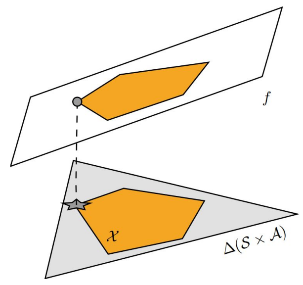
where $\mathbf{x} \in \mathbb{R}^{|\mathcal{S}| |\mathcal{A}|}$ and $\mathcal{X}$ is a convex set defined by a set of linear constraints. Hence, the problem above is a linear program, known as the dual formulation for MDPs. Intuitively, the result above tells us that searching over occupancies $\mathbf{d}_\pi$ is “equivalent” to searching over vectors $\mathbf{x}$ belonging to the set $\mathcal{X}$. Once the optimal solution $\mathbf{x}^* \in \mathcal{X}$ is found, we can retrieve the associated optimal policy via

$$\pi^*(a|s) = \frac{x^*(s,a)}{\sum_{a’ \in \mathcal{S}} x^*(s,a’)}.$$

We provide an illustration of this problem below.

What general-utility MDPs are all about

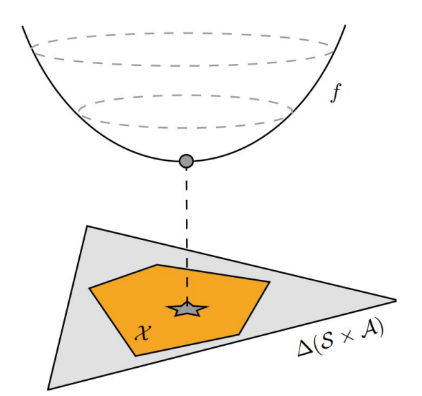
In GUMDPs, we are essentially building on top of the dual formulation for MDPs (and all associated fundamental resuts), and replacing the linear objective with a possibly non-linear function $f : \Delta(\mathcal{S} \times \mathcal{A}) \rightarrow \mathbb{R}$, where $\Delta(\mathcal{Z})$ denotes the set of probability distributions over a given set $\mathcal{Z}$. We then aim to solve

We illustrate this below.

Stationary policies suffice for optimality

Next, we describe some relevant objectives for GUMDPs.

3) Relevant objectives for GUMDPs

Many interesting problems can be formulated as GUMDPs. Some examples.

Standard MDPs:

where $\mathbf{c}$ is the vectorized cost function and we want to minimize the expected sum of discounted costs.

Exploration: Maximum state entropy exploration:

where we want to visit all states as randomly/uniformly as possible.

Imitation learning:

or

where $\mathbf{d}_\beta$ is the occupancy induced by the behavior policy $\beta$, and we want to match the frequency of visitation of states induced by policy $\beta$.

Diverse-skill discovery:

where we want to learn a set of $K$ policies $(\mathbf{d}^k_\pi)_{k=1}^K$ that are as diverse as possible.

4) How do we actually solve GUMDPs?

GUMDPs can be solved by:

• solving a sequence of non-stationary MDPs (Zahavy, 2023) (Geist, 2023).
• optimizing the policy via gradient descent on the objective (Kumar, 2023) (Zhang, 2020).

Approaches that involve solving a sequence of non-stationary MDPs resemble the application of the Frank-Wolfe algorithm for constrained optimization. We start at a given initial iterate $\mathbf{x}_0 \in \mathcal{X}$ and then iteratively update our iterate by solving a sequence of MDPs where the cost function, at each optimization step $t$, is given by the gradient of the objective $f$ evaluated at the current iterate, $\nabla f(\mathbf{x}_t)$. We illustrate this procedure below.

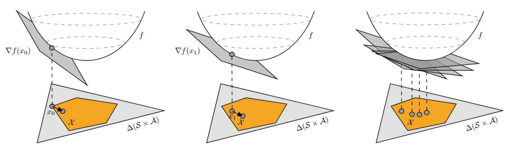
Approaches that perform gradient descent on the objective $f$ are essentially based on extensions of the policy gradient theorem to the case of objetive functions that depend on occupancies. Previous approaches considered parametrized policies $\pi_\theta$ and derived policy gradient theorems by exploiting the chain rule of calculus (Kumar, 2023) (Zhang, 2020).

What about continuous state/action spaces?

The framework of GUMDPs in its most standard form considers discrete state and action spaces. Naturally, it is interesting to explore the extension of similar ideas to the case of inherently continuous state and action spaces. Previous works extended the ideas herein discussed to the context of continuous state and action spaces by resorting to successor features.

Intuitively, the idea is to replace, for a given policy $\pi$, the expected frequency of visitation of state-action pairs $\mathbf{d}_\pi$, with the expected values of a set of features $\Phi = (\phi)_{k=1}^K$, with $\phi : \mathcal{S} \times \mathcal{A} \rightarrow \mathbb{R}$ and $K$ is usually much smaller than $| \mathcal{S}||\mathcal{A}|$. We then define the successor feature as

Finally, we define our objective in terms of the successor feature, aiming to find

This approach has been followed by previous works such as (Zahavy, 2024) (Leon, 2024).

References

(Geist, 2023) Geist, M., Pérolat, J., Laurière, M., Elie, R., Perrin, S., Bachem, O., … Pietquin, O. (2021). Concave Utility Reinforcement Learning: the Mean-field Game viewpoint. CoRR, abs/2106.03787.
(Kumar, 2023) Kumar, N., Wang, K., Levy, K., & Mannor, S. (2023). Policy Gradient for Reinforcement Learning with General Utilities. arXiv [Cs.LG].
(Leon, 2024) Leon, B. G., Riccio, F., Subramanian, K., Wurman, P. R., & Stone, P. (2024). Discovering Creative Behaviors through DUPLEX: Diverse Universal Features for Policy Exploration. In A. Globerson, L. Mackey, D. Belgrave, A. Fan, U. Paquet, J. Tomczak, & C. Zhang (Eds), Advances in Neural Information Processing Systems (Vol. 37, pp. 49625–49648). doi:10.52202/079017-1570
(Puterman, 2014) Puterman, M. L. (2014). Markov decision processes: discrete stochastic dynamic programming. John Wiley & Sons.
(Silver, 2021) Silver, D., Singh, S., Precup, D., & Sutton, R. S. (2021). Reward is enough. Artificial Intelligence, 299, 103535. doi:10.1016/j.artint.2021.103535
(Vamplew, 2021) Vamplew, P., Smith, B. J., Källström, J., de Oliveira Ramos, G., Radulescu, R., Roijers, D. M., … Foale, C. (2021). Scalar reward is not enough: A response to Silver, Singh, Precup and Sutton (2021). CoRR, abs/2112.15422.
(Zahavy, 2023) Zahavy, T., O’Donoghue, B., Desjardins, G., & Singh, S. (2023). Reward is enough for convex MDPs. arXiv [Cs.AI].
(Zahavy, 2024) Zahavy, T., Veeriah, V., Hou, S., Waugh, K., Lai, M., Leurent, E., … Singh, S. (2024). Diversifying AI: Towards Creative Chess with AlphaZero. arXiv [Cs.AI].
(Zhang, 2020) Zhang, J., Koppel, A., Bedi, A. S., Szepesvári, C., & Wang, M. (2020). Variational Policy Gradient Method for Reinforcement Learning with General Utilities. CoRR, abs/2007.02151
In this post we focus our attention to the case of cost functions but our discussion naturally carries to the case of reward functions. ↩︎
If the cost function is lower at a particular state (or set of states) than at all other possible states, then the agent will aim to move towards that (set of) state(s). If the cost function is equal at all states, all behaviors/policies are optimal. ↩︎